
In response to my post showing how to union two tables in Excel a reader writes,
I have seen your blog post about combining two tables, which I have working for me, however I would like to combine an ever increasing number of tables …, into a common “list”. How to do it without ending up with a nest IF statement beyond all control?!
We can avoid writing a deeply nested IF statement by creating a table that does some of the work for us.
The logic of the solution is the same as for the two table problem. A cell in the output table must ask,
- “Which table should I get my value from?” and
- “Which row should I get my value from?”
We create a helper table with this information in it.
First, let’s look at the work book, this has three tables to union, a helper table and an output table.

Below we see the “Tables to union” table,
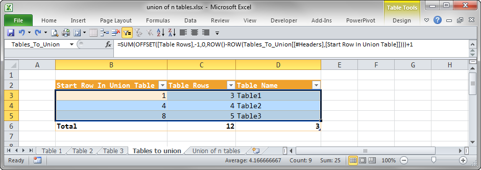
The table columns are
- Table Name: The names of the table in the union
- Table Rows: The number of rows in this table
- =ROWS(INDIRECT([@[Table Name]]))
- Start Row In Union Table:
- =SUM(OFFSET([Table Rows],-1,0,ROW()-ROW(Tables_To_Union[[#Headers],[Start Row In Union Table]])))+1
- This bizarre formula simply make a running total in Table Rows and adds 1.
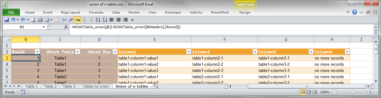
Each row in the union table can now simply lookup its value
- RowId =ROW(Table_union[@])-ROW(Table_union[[#Headers],[RowId]])
- Which Table =VLOOKUP([@RowId],Tables_To_Union,3,TRUE)
- Which Row =[@RowId]-VLOOKUP([@RowId],Tables_To_Union,1,TRUE)+1
- Column1 = =IFERROR(INDEX(INDIRECT([@[Which Table]]),[@[Which Row]],COLUMN()-COLUMN(Table_union[@])-2),”no more records”)
- Column2 =IFERROR(INDEX(INDIRECT([@[Which Table]]),[@[Which Row]],COLUMN()-COLUMN(Table_union[@])-2),”no more records”)
I think that this solution is quite elegant because it is easy to add additional tables and columns to the union and is reasonably readable. However when time allows I might write a custom function in VBA that uses the same logic.
I hope that you find this useful.

James, just to let you know that I’ve got this working and it meets my needs with a minimum of fuss, and no nested IF statements!! Many thanks for your help!.
I have the same problem but with a larger data set.
While pasting in your example code I cannot get it working.
Do you have a downloadable spreadsheet that I can use/edit?
Thanks for the assistance. Exactly what i was looking for to merge together tables.
Your use of @ and # are confusing to a beginner.
Dear Amy, Thank you for your comment. I think that the real issue is that this is a very hard problem to solve. If one day I find a simpler way I will post it. James