Power Query brings the power of ETL (extract, transform and load) tools to Excel. Almost every job I have now starts with using Power Query to clean and filter the data I am using.

But cleaning and filtering is only the most basic of Power Query’s functionality. It can also be used to calculate custom columns and in some circumstances this can be a less fragile solution than doing calculations to the cleaned data in a worksheet.

For a recent job it was necessary to calculate a running total (cumulative total) of stock in and stock out (sales & expenses). This is a very common challenge so thought I would learn to do it in Power Query.

There is a great training video here which also demonstrates higher performance solutions that the one I present below.

If you are familiar with creating custom columns you will find it easy. The one “gotcha” for me was that I did not understand that each step in Power Query creates a new table with the name of the step. I have annotated a screenshot to show you how to do it.

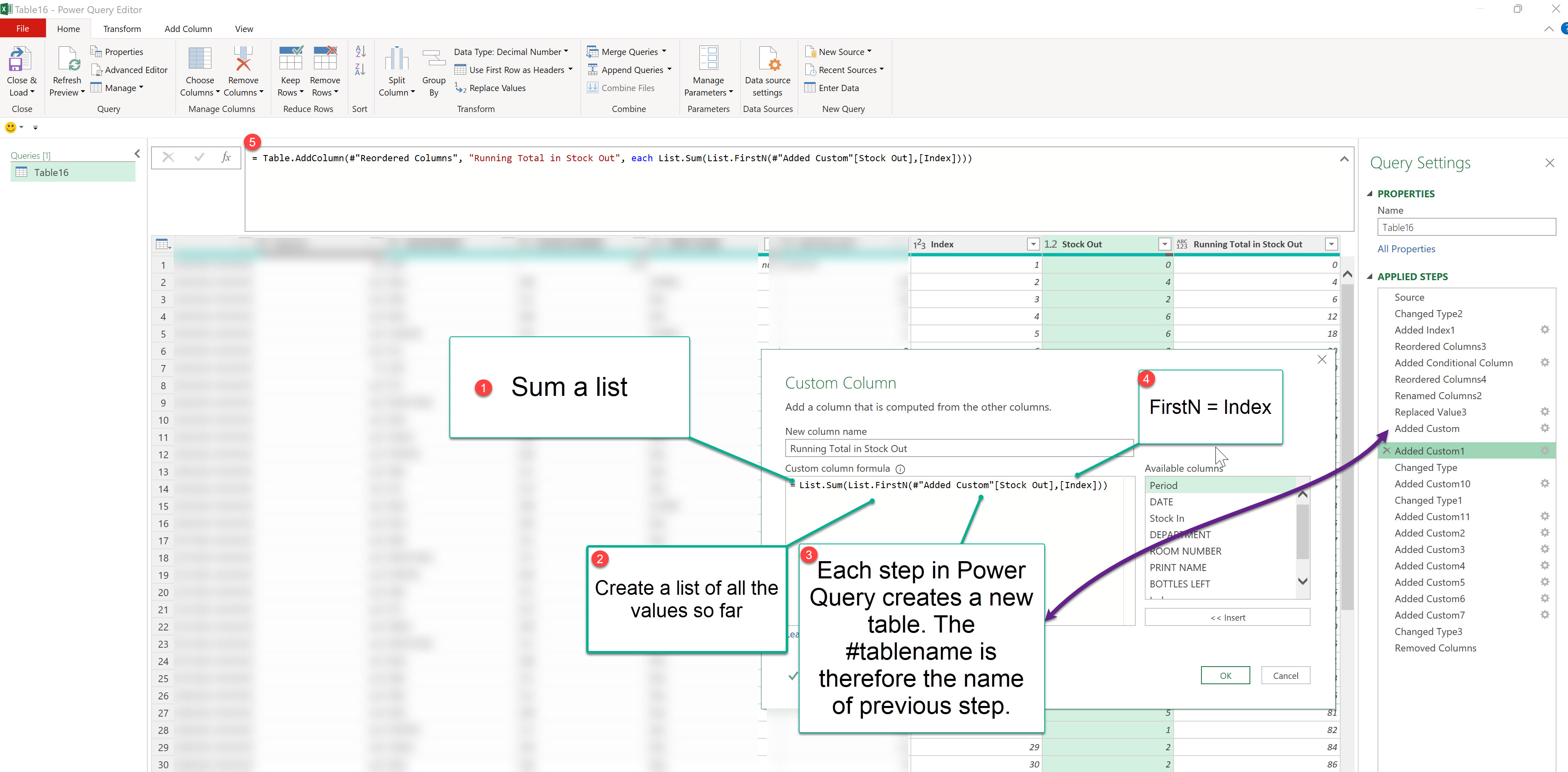
1. We will sum a list
2. We create a list of the values so far using List.FirstN()
3. The source list of the List.FirstN() is the [Stock Out] column in the previous step. This is referenced as #”Added Custom”[Stock Out] because the previous step was called “Added Custom”.
4. The number of list elements to include “FirstN” is defined by the length of the list which is given by the value of the Index column. This parameter can also be used as filter, look at the definition of List.FirstN() for more details.

I hope that you found this useful and welcome your comments.

(See also Power Query SumIf)